 Data Science
Chapter 11 Combining code and text with Jupyter
11.1 Overview
A typical data analysis involves not only writing and executing code, but also writing text and displaying images that help tell the story of the analysis. In fact, ideally, we would like to interleave these three media, with the text and images serving as narration for the code and its output. In this chapter we will show you how to accomplish this using Jupyter notebooks, a common coding platform in data science. Jupyter notebooks do precisely what we need: they let you combine text, images, and (executable!) code in a single document. In this chapter, we will focus on the use of Jupyter notebooks to program in R and write text via a web interface. These skills are essential to getting your analysis running; think of it like getting dressed in the morning! Note that we assume that you already have Jupyter set up and ready to use. If that is not the case, please first read Chapter 13 to learn how to install and configure Jupyter on your own computer.
11.2 Chapter learning objectives
By the end of the chapter, readers will be able to do the following:
- Create new Jupyter notebooks.
- Write, edit, and execute R code in a Jupyter notebook.
- Write, edit, and view text in a Jupyter notebook.
- Open and view plain text data files in Jupyter.
- Export Jupyter notebooks to other standard file types (e.g.,
.html,.pdf).
11.3 Jupyter
Jupyter (Kluyver et al. 2016) is a web-based interactive development environment for creating, editing, and executing documents called Jupyter notebooks. Jupyter notebooks are documents that contain a mix of computer code (and its output) and formattable text. Given that they combine these two analysis artifacts in a single document—code is not separate from the output or written report—notebooks are one of the leading tools to create reproducible data analyses. Reproducible data analysis is one where you can reliably and easily re-create the same results when analyzing the same data. Although this sounds like something that should always be true of any data analysis, in reality, this is not often the case; one needs to make a conscious effort to perform data analysis in a reproducible manner. An example of what a Jupyter notebook looks like is shown in Figure 11.1.
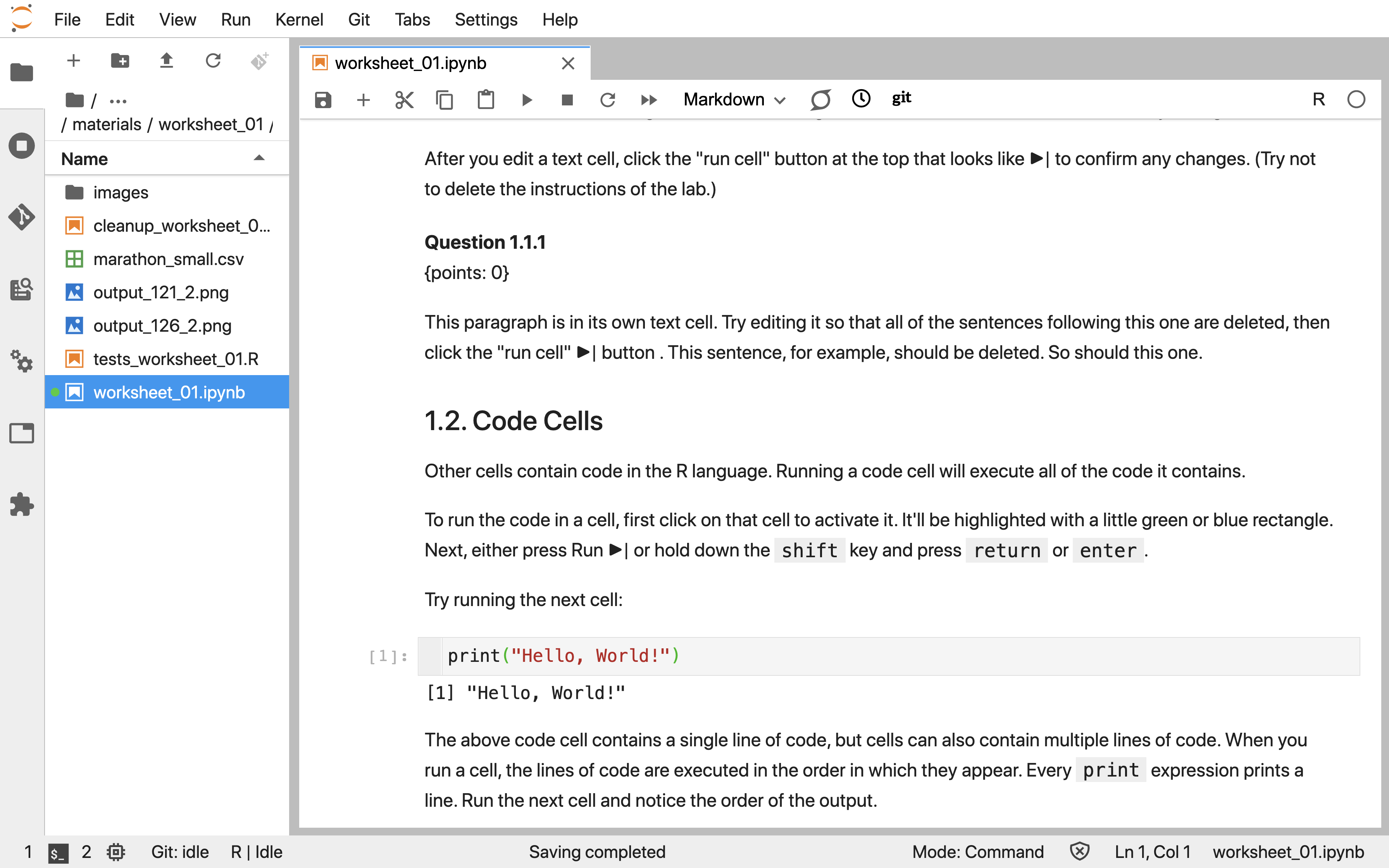
Figure 11.1: A screenshot of a Jupyter Notebook.
11.3.1 Accessing Jupyter
One of the easiest ways to start working with Jupyter is to use a web-based platform called JupyterHub. JupyterHubs often have Jupyter, R, a number of R packages, and collaboration tools installed, configured and ready to use. JupyterHubs are usually created and provisioned by organizations, and require authentication to gain access. For example, if you are reading this book as part of a course, your instructor may have a JupyterHub already set up for you to use! Jupyter can also be installed on your own computer; see Chapter 13 for instructions.
11.4 Code cells
The sections of a Jupyter notebook that contain code are referred to as code cells. A code cell that has not yet been executed has no number inside the square brackets to the left of the cell (Figure 11.2). Running a code cell will execute all of the code it contains, and the output (if any exists) will be displayed directly underneath the code that generated it. Outputs may include printed text or numbers, data frames and data visualizations. Cells that have been executed also have a number inside the square brackets to the left of the cell. This number indicates the order in which the cells were run (Figure 11.3).
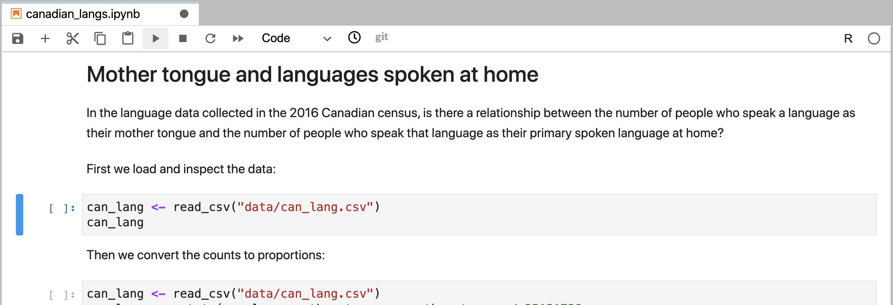
Figure 11.2: A code cell in Jupyter that has not yet been executed.
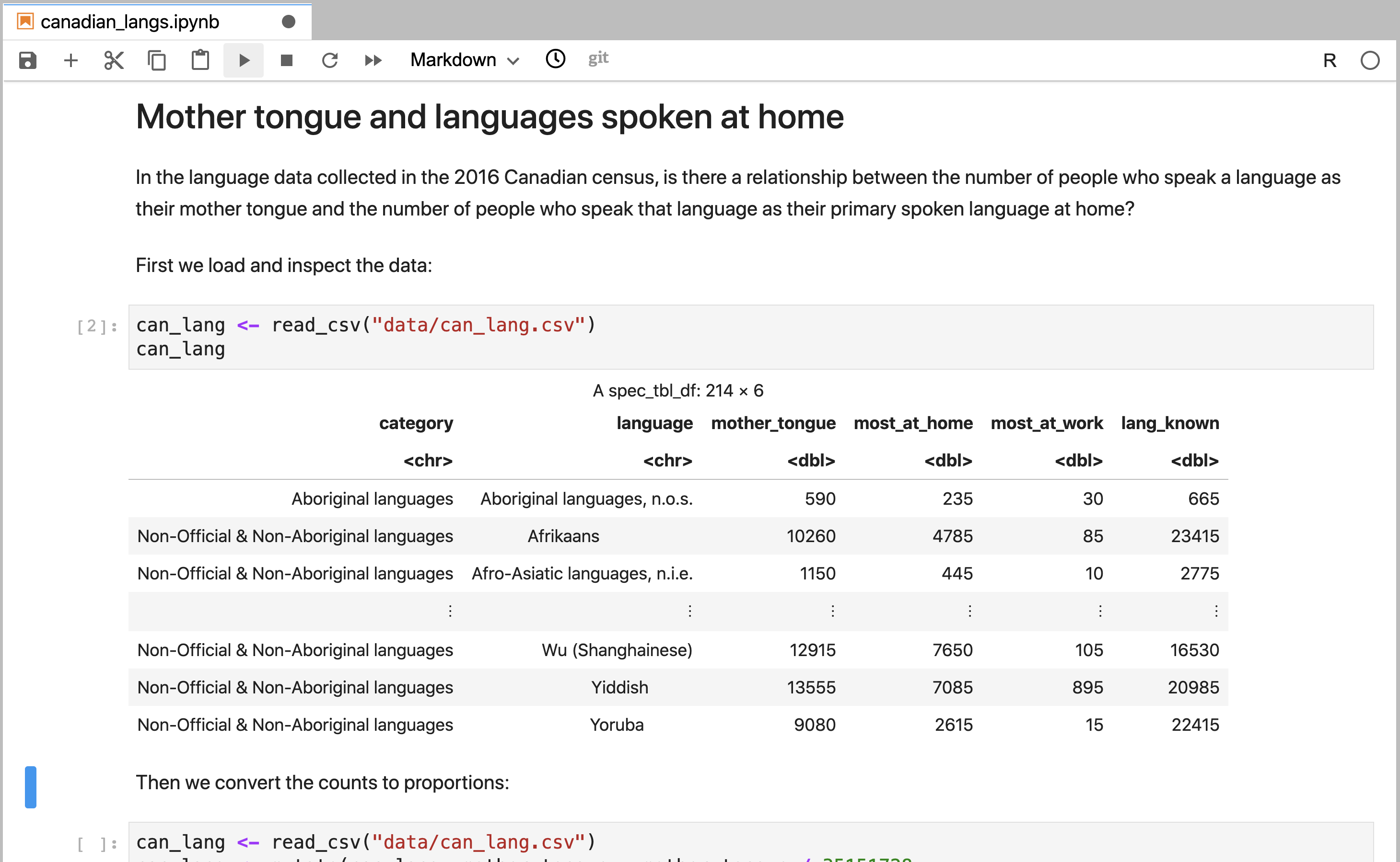
Figure 11.3: A code cell in Jupyter that has been executed.
11.4.1 Executing code cells
Code cells can be run independently or as part of executing the entire notebook using one of the “Run all” commands found in the Run or Kernel menus in Jupyter. Running a single code cell independently is a workflow typically used when editing or writing your own R code. Executing an entire notebook is a workflow typically used to ensure that your analysis runs in its entirety before sharing it with others, and when using a notebook as part of an automated process.
To run a code cell independently, the cell needs to first be activated. This
is done by clicking on it with the cursor. Jupyter will indicate a cell has been
activated by highlighting it with a blue rectangle to its left. After the cell
has been activated (Figure 11.4), the cell can be run
by either pressing the Run (▶).
button in the toolbar, or by using the keyboard shortcut Shift + Enter.
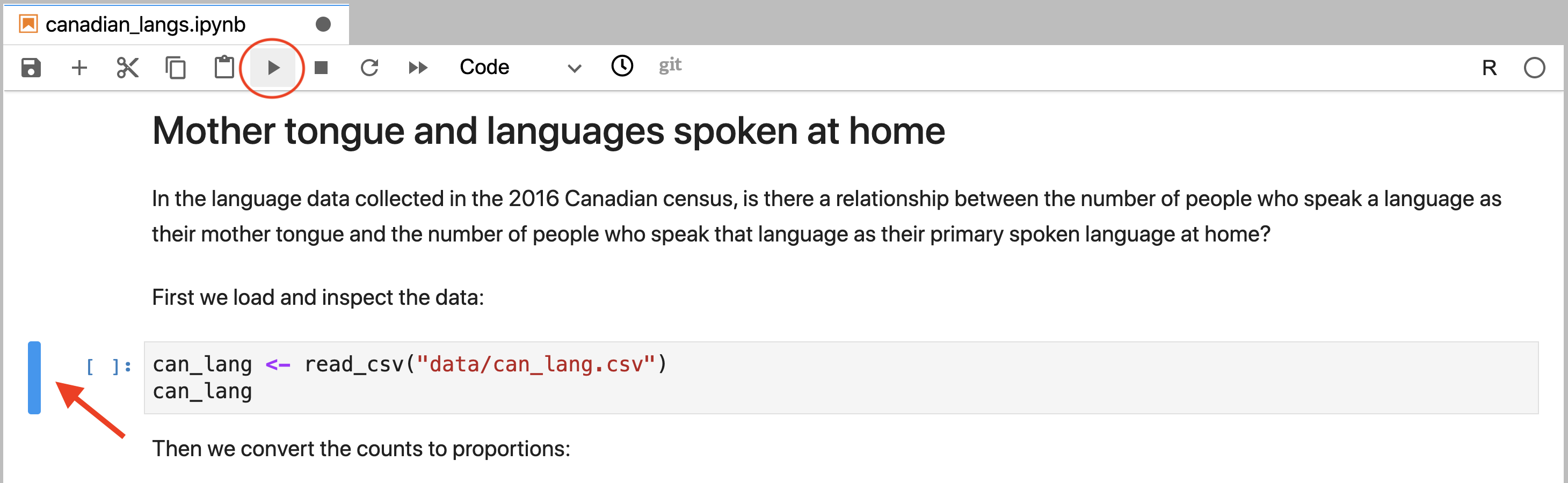
Figure 11.4: An activated cell that is ready to be run. The blue rectangle to the cell’s left (annotated by a red arrow) indicates that it is ready to be run. The cell can be run by clicking the run button (circled in red).
To execute all of the code cells in an entire notebook, you have three options:
Select Run >> Run All Cells from the menu.
Select Kernel >> Restart Kernel and Run All Cells… from the menu (Figure 11.5).
Click the (⏭) button in the tool bar.
All of these commands result in all of the code cells in a notebook being run. However, there is a slight difference between them. In particular, only options 2 and 3 above will restart the R session before running all of the cells; option 1 will not restart the session. Restarting the R session means that all previous objects that were created from running cells before this command was run will be deleted. In other words, restarting the session and then running all cells (options 2 or 3) emulates how your notebook code would run if you completely restarted Jupyter before executing your entire notebook.
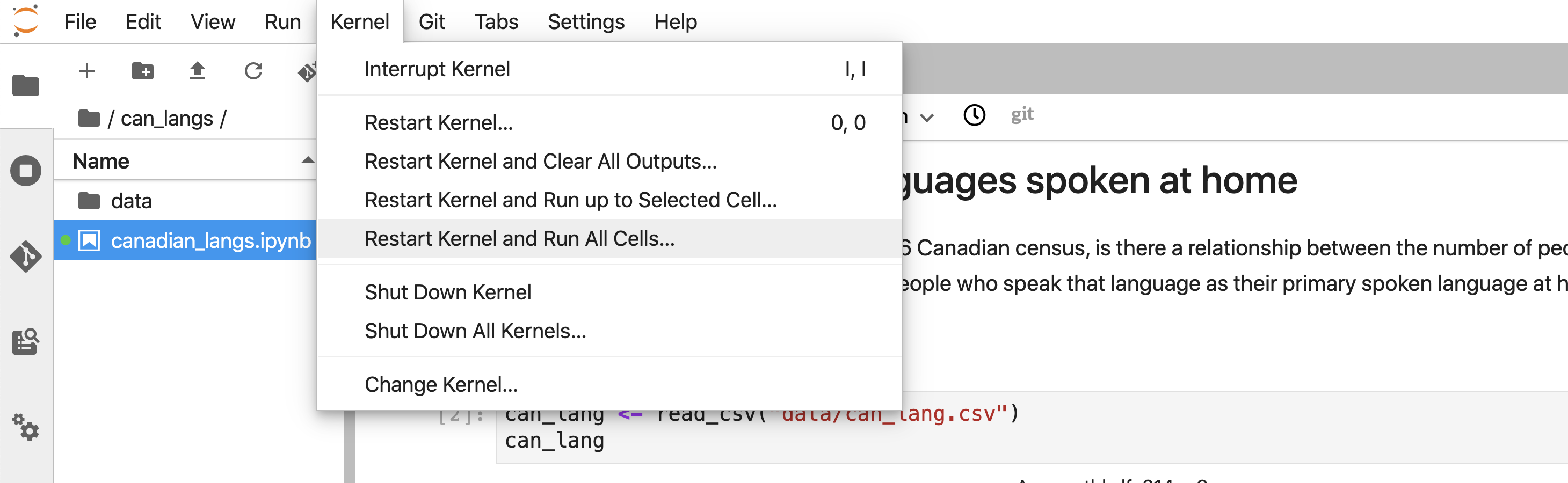
Figure 11.5: Restarting the R session can be accomplished by clicking Restart Kernel and Run All Cells…
11.4.2 The Kernel
The kernel is a program that executes the code inside your notebook and outputs the results. Kernels for many different programming languages have been created for Jupyter, which means that Jupyter can interpret and execute the code of many different programming languages. To run R code, your notebook will need an R kernel. In the top right of your window, you can see a circle that indicates the status of your kernel. If the circle is empty (◯) the kernel is idle and ready to execute code. If the circle is filled in (⬤) the kernel is busy running some code.
You may run into problems where your kernel is stuck for an excessive amount of time, your notebook is very slow and unresponsive, or your kernel loses its connection. If this happens, try the following steps:
- At the top of your screen, click Kernel, then Interrupt Kernel.
- If that doesn’t help, click Kernel, then Restart Kernel… If you do this, you will have to run your code cells from the start of your notebook up until where you paused your work.
- If that still doesn’t help, restart Jupyter. First, save your work by clicking File at the top left of your screen, then Save Notebook. Next, if you are accessing Jupyter using a JupyterHub server, from the File menu click Hub Control Panel. Choose Stop My Server to shut it down, then the My Server button to start it back up. If you are running Jupyter on your own computer, from the File menu click Shut Down, then start Jupyter again. Finally, navigate back to the notebook you were working on.
11.4.3 Creating new code cells
To create a new code cell in Jupyter (Figure 11.6), click the + button in the
toolbar. By default, all new cells in Jupyter start out as code cells,
so after this, all you have to do is write R code within the new cell you just
created!
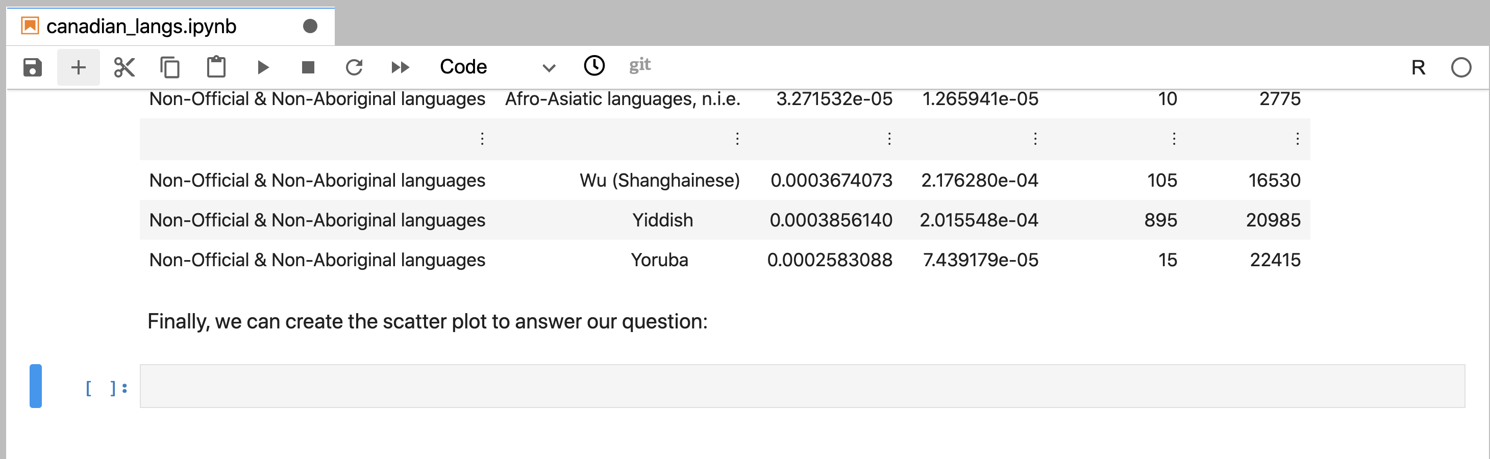
Figure 11.6: New cells can be created by clicking the + button, and are by default code cells.
11.5 Markdown cells
Text cells inside a Jupyter notebook are called Markdown cells. Markdown cells are rich formatted text cells, which means you can bold and italicize text, create subject headers, create bullet and numbered lists, and more. These cells are given the name “Markdown” because they use Markdown language to specify the rich text formatting. You do not need to learn Markdown to write text in the Markdown cells in Jupyter; plain text will work just fine. However, you might want to learn a bit about Markdown eventually to enable you to create nicely formatted analyses. See the additional resources at the end of this chapter to find out where you can start learning Markdown.
11.5.1 Editing Markdown cells
To edit a Markdown cell in Jupyter, you need to double click on the cell. Once
you do this, the unformatted (or unrendered) version of the text will be
shown (Figure 11.7). You
can then use your keyboard to edit the text. To view the formatted
(or rendered) text (Figure 11.8), click the Run (▶) button in the toolbar,
or use the Shift + Enter keyboard shortcut.
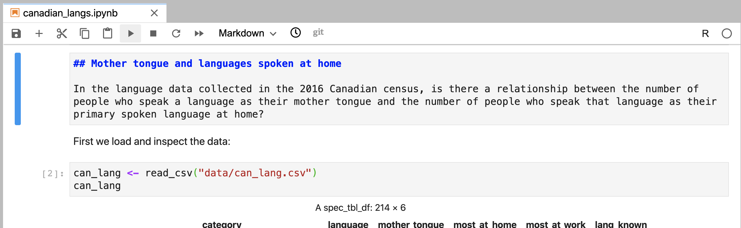
Figure 11.7: A Markdown cell in Jupyter that has not yet been rendered and can be edited.
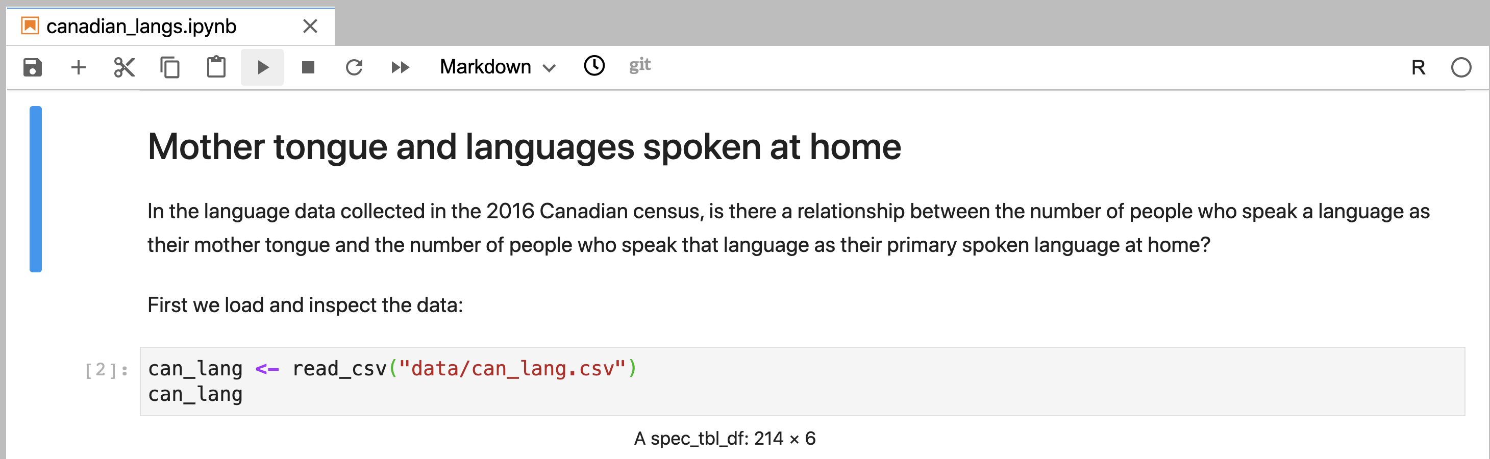
Figure 11.8: A Markdown cell in Jupyter that has been rendered and exhibits rich text formatting.
11.5.2 Creating new Markdown cells
To create a new Markdown cell in Jupyter, click the + button in the toolbar.
By default, all new cells in Jupyter start as code cells, so
the cell format needs to be changed to be recognized and rendered as a Markdown
cell. To do this, click on the cell with your cursor to
ensure it is activated. Then click on the drop-down box on the toolbar that says “Code” (it
is next to the ⏭ button), and change it from “Code” to “Markdown” (Figure 11.9).
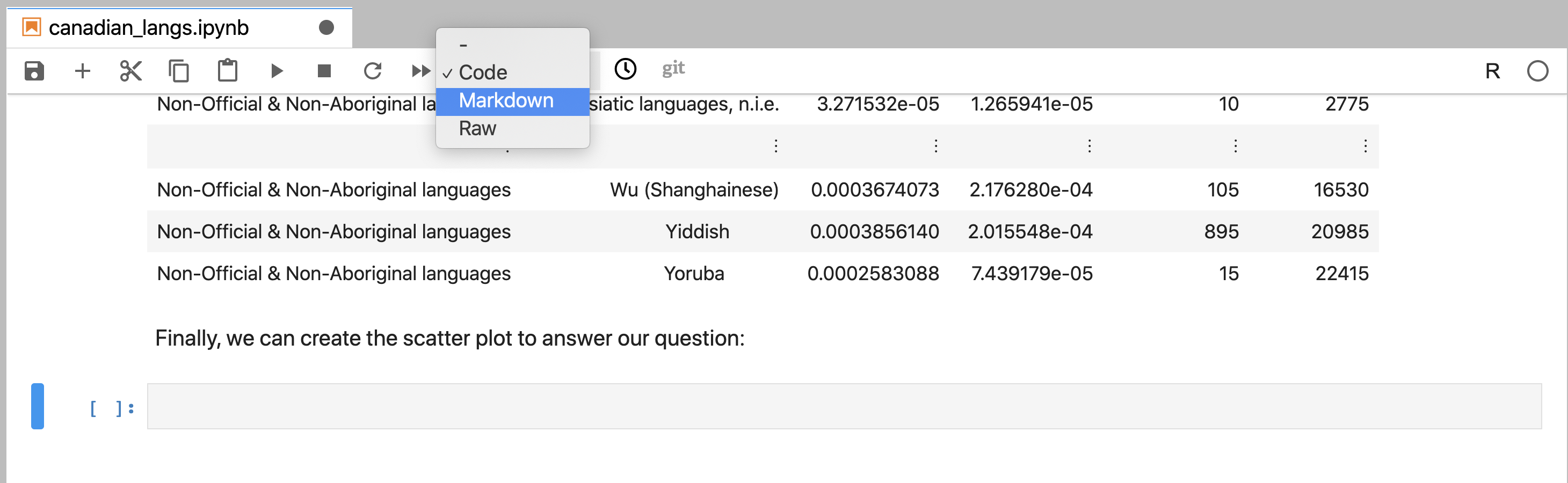
Figure 11.9: New cells are by default code cells. To create Markdown cells, the cell format must be changed.
11.6 Saving your work
As with any file you work on, it is critical to save your work often so you
don’t lose your progress! Jupyter has an autosave feature, where open files are
saved periodically. The default for this is every two minutes. You can also
manually save a Jupyter notebook by selecting Save Notebook from the
File menu, by clicking the disk icon on the toolbar,
or by using a keyboard shortcut (Control + S for Windows, or Command + S for
Mac OS).
11.7 Best practices for running a notebook
11.7.1 Best practices for executing code cells
As you might know (or at least imagine) by now, Jupyter notebooks are great for interactively editing, writing and running R code; this is what they were designed for! Consequently, Jupyter notebooks are flexible in regards to code cell execution order. This flexibility means that code cells can be run in any arbitrary order using the Run (▶) button. But this flexibility has a downside: it can lead to Jupyter notebooks whose code cannot be executed in a linear order (from top to bottom of the notebook). A nonlinear notebook is problematic because a linear order is the conventional way code documents are run, and others will have this expectation when running your notebook. Finally, if the code is used in some automated process, it will need to run in a linear order, from top to bottom of the notebook.
The most common way to inadvertently create a nonlinear notebook is to rely solely
on using the ▶ button to execute cells. For example,
suppose you write some R code that creates an R object, say a variable named
y. When you execute that cell and create y, it will continue
to exist until it is deliberately deleted with R code, or when the Jupyter
notebook R session (i.e., kernel) is stopped or restarted. It can also be
referenced in another distinct code cell (Figure 11.10).
Together, this means that you could then write a code cell further above in the
notebook that references y and execute it without error in the current session
(Figure 11.11). This could also be done successfully in
future sessions if, and only if, you run the cells in the same unconventional
order. However, it is difficult to remember this unconventional order, and it
is not the order that others would expect your code to be executed in. Thus, in
the future, this would lead
to errors when the notebook is run in the conventional
linear order (Figure 11.12).
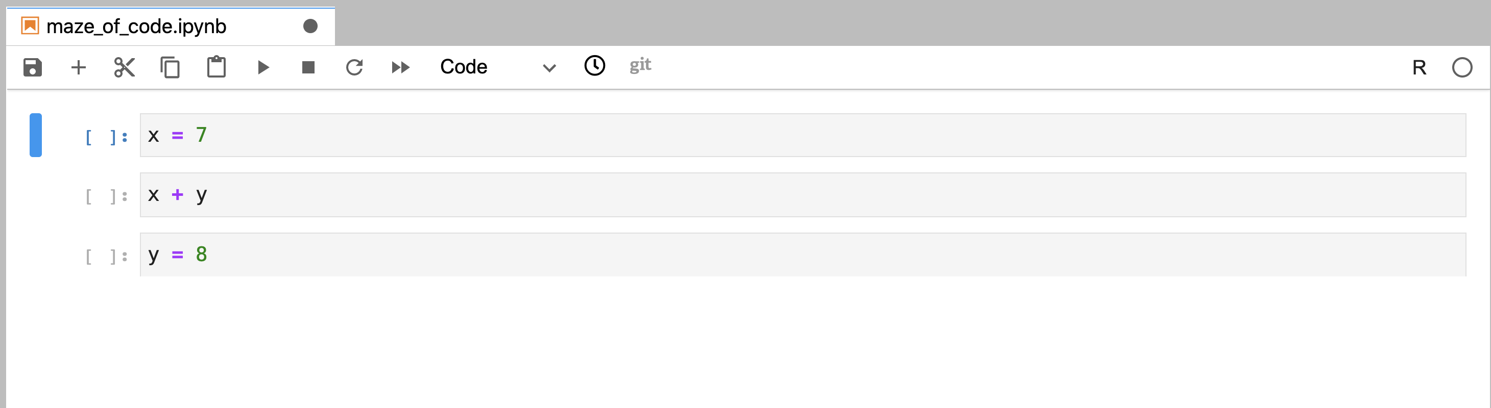
Figure 11.10: Code that was written out of order, but not yet executed.
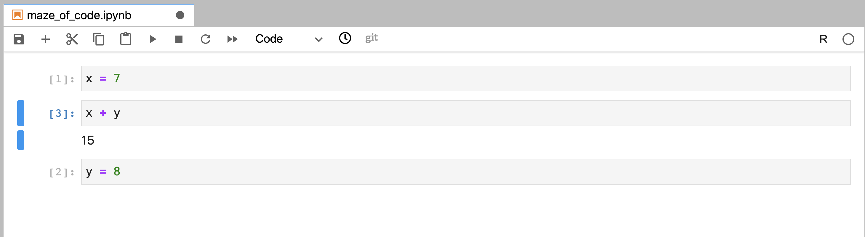
Figure 11.11: Code that was written out of order, and was executed using the run button in a nonlinear order without error. The order of execution can be traced by following the numbers to the left of the code cells; their order indicates the order in which the cells were executed.
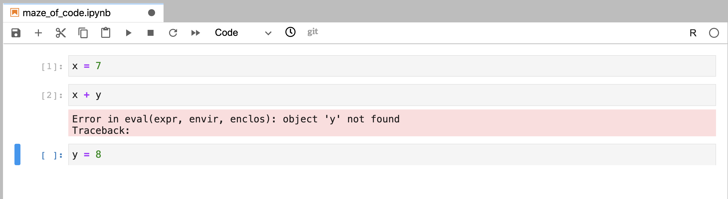
Figure 11.12: Code that was written out of order, and was executed in a linear order using “Restart Kernel and Run All Cells…” This resulted in an error at the execution of the second code cell and it failed to run all code cells in the notebook.
You can also accidentally create a nonfunctioning notebook by creating an object in a cell that later gets deleted. In such a scenario, that object only exists for that one particular R session and will not exist once the notebook is restarted and run again. If that object was referenced in another cell in that notebook, an error would occur when the notebook was run again in a new session.
These events may not negatively affect the current R session when the code is being written; but as you might now see, they will likely lead to errors when that notebook is run in a future session. Regularly executing the entire notebook in a fresh R session will help guard against this. If you restart your session and new errors seem to pop up when you run all of your cells in linear order, you can at least be aware that there is an issue. Knowing this sooner rather than later will allow you to fix the issue and ensure your notebook can be run linearly from start to finish.
We recommend as a best practice to run the entire notebook in a fresh R session at least 2–3 times within any period of work. Note that, critically, you must do this in a fresh R session by restarting your kernel. We recommend using either the Kernel >> Restart Kernel and Run All Cells… command from the menu or the ⏭ button in the toolbar. Note that the Run >> Run All Cells menu item will not restart the kernel, and so it is not sufficient to guard against these errors.
11.7.2 Best practices for including R packages in notebooks
Most data analyses these days depend on functions from external R packages that
are not built into R. One example is the tidyverse metapackage that we
heavily rely on in this book. This package provides us access to functions like
read_csv for reading data, select for subsetting columns, and ggplot for
creating high-quality graphics.
As mentioned earlier in the book, external R packages need to be loaded before
the functions they contain can be used. Our recommended way to do this is via
library(package_name). But where should this line of code be written in a
Jupyter notebook? One idea could be to load the library right before the
function is used in the notebook. However, although this technically works, this
causes hidden, or at least non-obvious, R package dependencies when others view
or try to run the notebook. These hidden dependencies can lead to errors when
the notebook is executed on another computer if the needed R packages are not
installed. Additionally, if the data analysis code takes a long time to run,
uncovering the hidden dependencies that need to be installed so that the
analysis can run without error can take a great deal of time to uncover.
Therefore, we recommend you load all R packages in a code cell near the top of the Jupyter notebook. Loading all your packages at the start ensures that all packages are loaded before their functions are called, assuming the notebook is run in a linear order from top to bottom as recommended above. It also makes it easy for others viewing or running the notebook to see what external R packages are used in the analysis, and hence, what packages they should install on their computer to run the analysis successfully.
11.7.3 Summary of best practices for running a notebook
Write code so that it can be executed in a linear order.
As you write code in a Jupyter notebook, run the notebook in a linear order and in its entirety often (2–3 times every work session) via the Kernel >> Restart Kernel and Run All Cells… command from the Jupyter menu or the ⏭ button in the toolbar.
Write the code that loads external R packages near the top of the Jupyter notebook.
11.8 Exploring data files
It is essential to preview data files before you try to read them into R to see whether or not there are column names, what the delimiters are, and if there are lines you need to skip. In Jupyter, you preview data files stored as plain text files (e.g., comma- and tab-separated files) in their plain text format (Figure 11.14) by right-clicking on the file’s name in the Jupyter file explorer, selecting Open with, and then selecting Editor (Figure 11.13). Suppose you do not specify to open the data file with an editor. In that case, Jupyter will render a nice table for you, and you will not be able to see the column delimiters, and therefore you will not know which function to use, nor which arguments to use and values to specify for them.
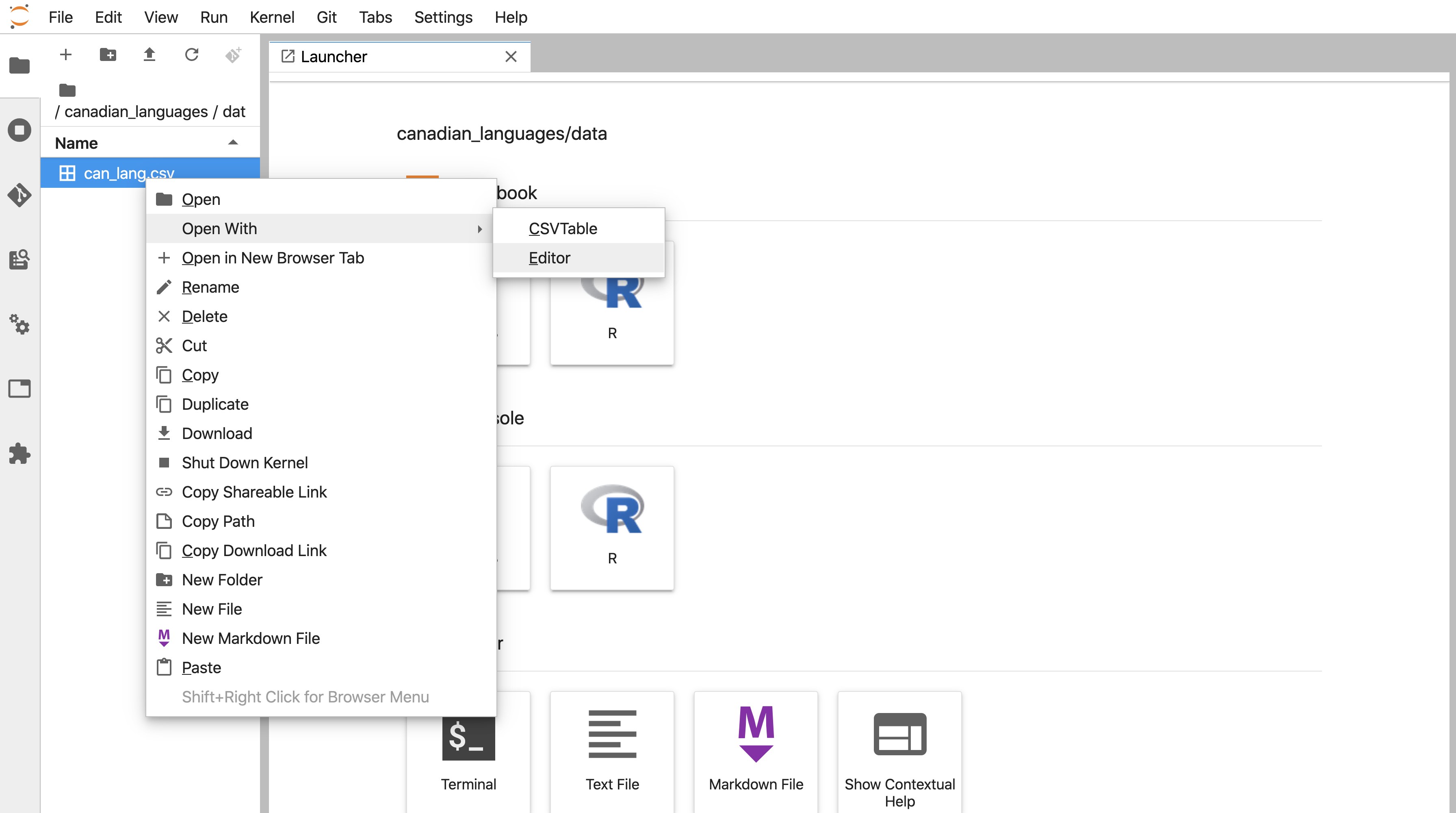
Figure 11.13: Opening data files with an editor in Jupyter.
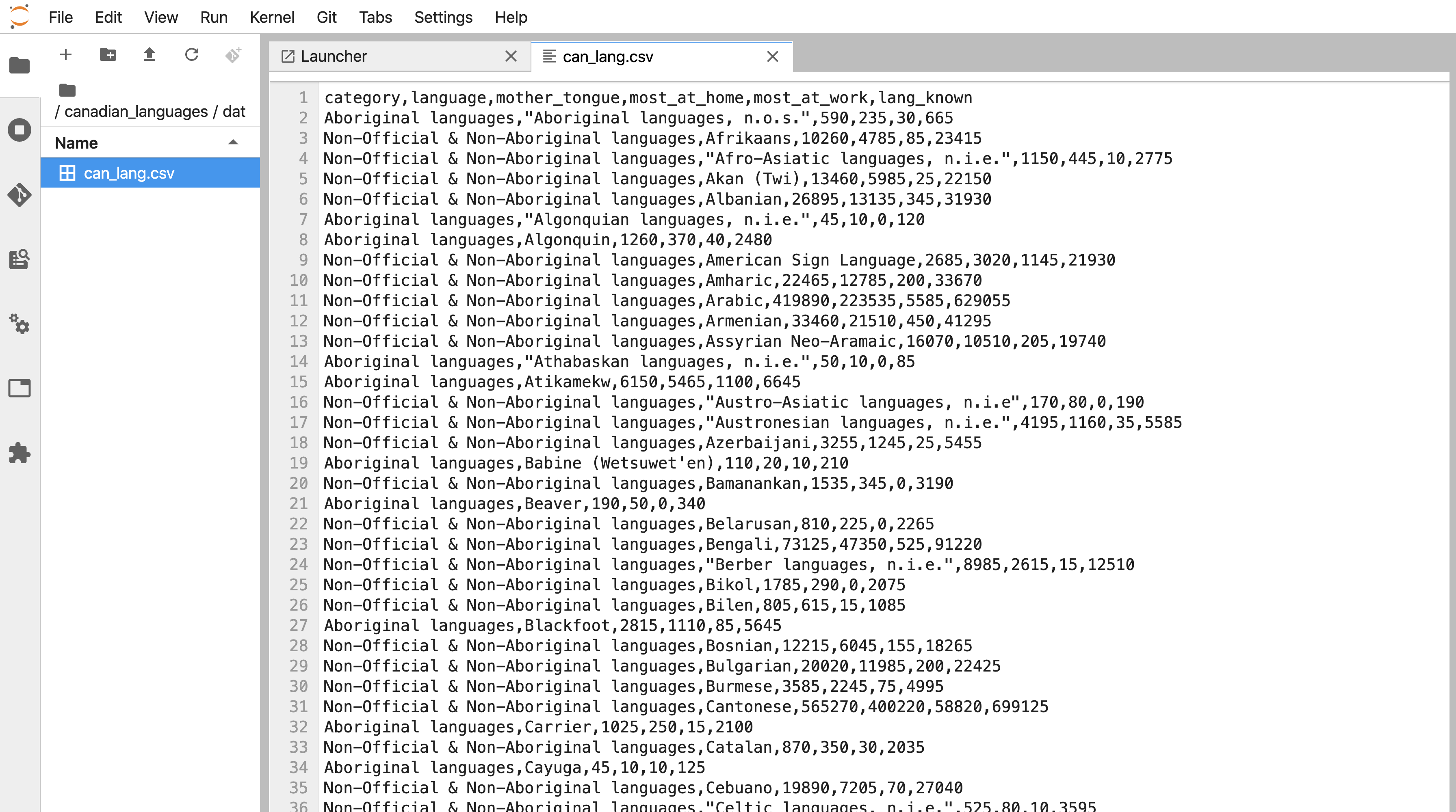
Figure 11.14: A data file as viewed in an editor in Jupyter.
11.9 Exporting to a different file format
In Jupyter, viewing, editing and running R code is done in the Jupyter notebook
file format with file extension .ipynb. This file format is not easy to open and
view outside of Jupyter. Thus, to share your analysis with people who do not
commonly use Jupyter, it is recommended that you export your executed analysis
as a more common file type, such as an .html file, or a .pdf. We recommend
exporting the Jupyter notebook after executing the analysis so that you can
also share the outputs of your code. Note, however, that your audience will not be
able to run your analysis using a .html or .pdf file. If you want your audience
to be able to reproduce the analysis, you must provide them with the .ipynb Jupyter notebook file.
11.9.1 Exporting to HTML
Exporting to .html will result in a shareable file that anyone can open
using a web browser (e.g., Firefox, Safari, Chrome, or Edge). The .html
output will produce a document that is visually similar to what the Jupyter notebook
looked like inside Jupyter. One point of caution here is that if there are
images in your Jupyter notebook, you will need to share the image files and the
.html file to see them.
11.9.2 Exporting to PDF
Exporting to .pdf will result in a shareable file that anyone can open
using many programs, including Adobe Acrobat, Preview, web browsers and many
more. The benefit of exporting to PDF is that it is a standalone document,
even if the Jupyter notebook included references to image files.
Unfortunately, the default settings will result in a document
that visually looks quite different from what the Jupyter notebook looked
like. The font, page margins, and other details will appear different in the .pdf output.
11.10 Creating a new Jupyter notebook
At some point, you will want to create a new, fresh Jupyter notebook for your own project instead of viewing, running or editing a notebook that was started by someone else. To do this, navigate to the Launcher tab, and click on the R icon under the Notebook heading. If no Launcher tab is visible, you can get a new one via clicking the + button at the top of the Jupyter file explorer (Figure 11.15).
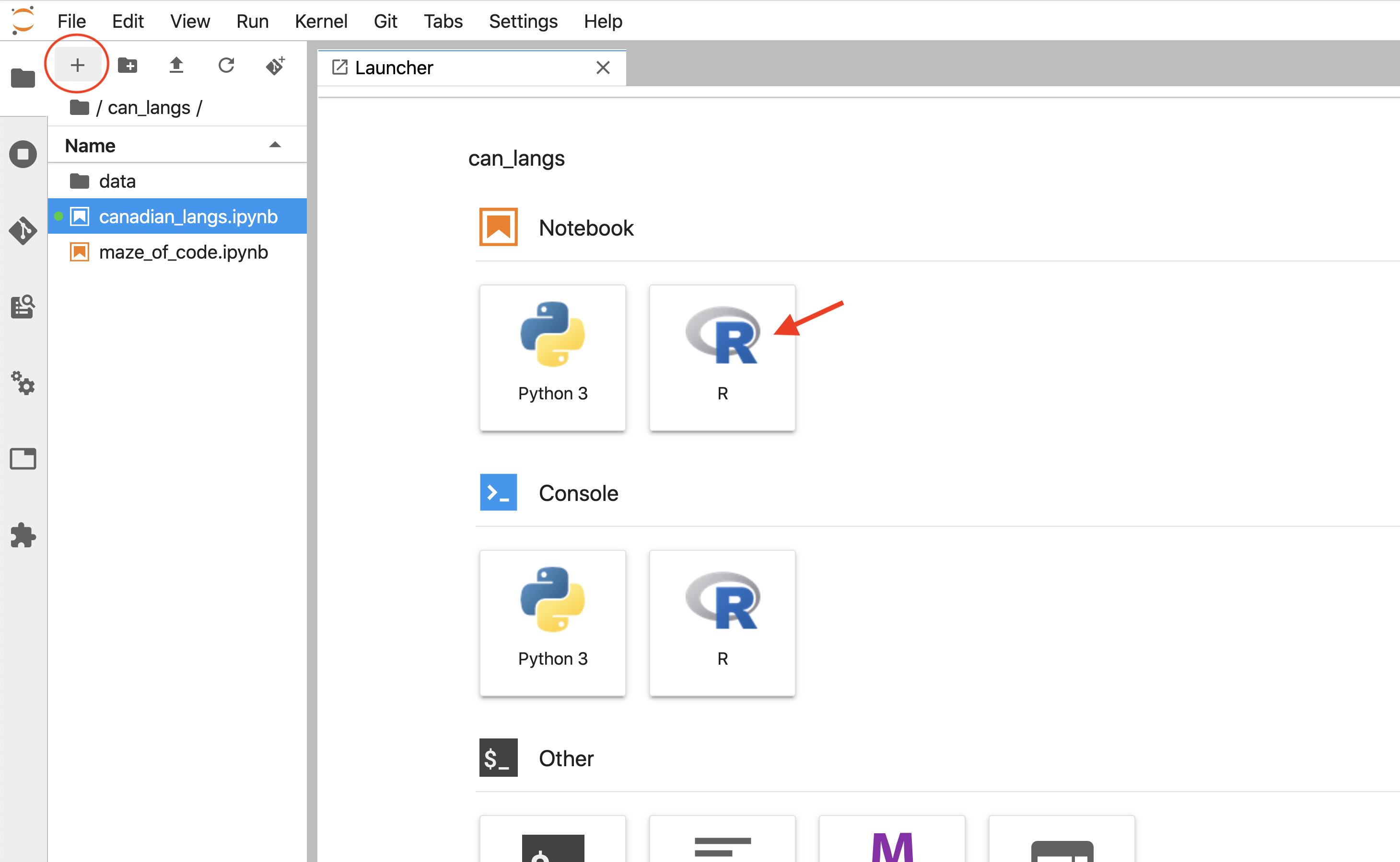
Figure 11.15: Clicking on the R icon under the Notebook heading will create a new Jupyter notebook with an R kernel.
Once you have created a new Jupyter notebook, be sure to give it a descriptive
name, as the default file name is Untitled.ipynb. You can rename files by
first right-clicking on the file name of the notebook you just created, and
then clicking Rename. This will make
the file name editable. Use your keyboard to
change the name. Pressing Enter or clicking anywhere else in the Jupyter
interface will save the changed file name.
We recommend not using white space or non-standard characters in file names.
Doing so will not prevent you from using that file in Jupyter. However, these
sorts of things become troublesome as you start to do more advanced data
science projects that involve repetition and automation. We recommend naming
files using lower case characters and separating words by a dash (-) or an
underscore (_).
11.11 Additional resources
- The JupyterLab Documentation is a good next place to look for more information about working in Jupyter notebooks. This documentation goes into significantly more detail about all of the topics we covered in this chapter, and covers more advanced topics as well.
- If you are keen to learn about the Markdown language for rich text formatting, two good places to start are CommonMark’s Markdown cheatsheet and Markdown tutorial.