Chapter 7 Regression I: K-nearest neighbors
7.1 Overview
This chapter continues our foray into answering predictive questions.
Here we will focus on predicting numerical variables
and will use regression to perform this task.
This is unlike the past two chapters, which focused on predicting categorical
variables via classification. However, regression does have many similarities
to classification: for example, just as in the case of classification,
we will split our data into training, validation, and test sets, we will
use tidymodels workflows, we will use a K-nearest neighbors (K-NN)
approach to make predictions, and we will use cross-validation to choose K.
Because of how similar these procedures are, make sure to read Chapters
5 and 6 before reading
this one—we will move a little bit faster here with the
concepts that have already been covered.
This chapter will primarily focus on the case where there is a single predictor,
but the end of the chapter shows how to perform
regression with more than one predictor variable, i.e., multivariable regression.
It is important to note that regression
can also be used to answer inferential and causal questions,
however that is beyond the scope of this book.
7.2 Chapter learning objectives
By the end of the chapter, readers will be able to do the following:
- Recognize situations where a regression analysis would be appropriate for making predictions.
- Explain the K-nearest neighbors (K-NN) regression algorithm and describe how it differs from K-NN classification.
- Interpret the output of a K-NN regression.
- In a data set with two or more variables, perform K-nearest neighbors regression in R.
- Evaluate K-NN regression prediction quality in R using the root mean squared prediction error (RMSPE).
- Estimate the RMSPE in R using cross-validation or a test set.
- Choose the number of neighbors in K-nearest neighbors regression by minimizing estimated cross-validation RMSPE.
- Describe underfitting and overfitting, and relate it to the number of neighbors in K-nearest neighbors regression.
- Describe the advantages and disadvantages of K-nearest neighbors regression.
7.3 The regression problem
Regression, like classification, is a predictive problem setting where we want to use past information to predict future observations. But in the case of regression, the goal is to predict numerical values instead of categorical values. The variable that you want to predict is often called the response variable. For example, we could try to use the number of hours a person spends on exercise each week to predict their race time in the annual Boston marathon. As another example, we could try to use the size of a house to predict its sale price. Both of these response variables—race time and sale price—are numerical, and so predicting them given past data is considered a regression problem.
Just like in the classification setting, there are many possible methods that we can use to predict numerical response variables. In this chapter we will focus on the K-nearest neighbors algorithm (Fix and Hodges 1951; Cover and Hart 1967), and in the next chapter we will study linear regression. In your future studies, you might encounter regression trees, splines, and general local regression methods; see the additional resources section at the end of the next chapter for where to begin learning more about these other methods.
Many of the concepts from classification map over to the setting of regression. For example, a regression model predicts a new observation’s response variable based on the response variables for similar observations in the data set of past observations. When building a regression model, we first split the data into training and test sets, in order to ensure that we assess the performance of our method on observations not seen during training. And finally, we can use cross-validation to evaluate different choices of model parameters (e.g., K in a K-nearest neighbors model). The major difference is that we are now predicting numerical variables instead of categorical variables.
Note: You can usually tell whether a variable is numerical or categorical—and therefore whether you need to perform regression or classification—by taking the response variable for two observations X and Y from your data, and asking the question, “is response variable X more than response variable Y?” If the variable is categorical, the question will make no sense. (Is blue more than red? Is benign more than malignant?) If the variable is numerical, it will make sense. (Is 1.5 hours more than 2.25 hours? Is $500,000 more than $400,000?) Be careful when applying this heuristic, though: sometimes categorical variables will be encoded as numbers in your data (e.g., “1” represents “benign”, and “0” represents “malignant”). In these cases you have to ask the question about the meaning of the labels (“benign” and “malignant”), not their values (“1” and “0”).
7.4 Exploring a data set
In this chapter and the next, we will study a data set of 932 real estate transactions in Sacramento, California originally reported in the Sacramento Bee newspaper. We first need to formulate a precise question that we want to answer. In this example, our question is again predictive: Can we use the size of a house in the Sacramento, CA area to predict its sale price? A rigorous, quantitative answer to this question might help a realtor advise a client as to whether the price of a particular listing is fair, or perhaps how to set the price of a new listing. We begin the analysis by loading and examining the data, and setting the seed value.
library(tidyverse)
library(tidymodels)
library(gridExtra)

set.seed(5)

sacramento <- read_csv("data/sacramento.csv")
sacramento
## # A tibble: 932 × 9
## city zip beds baths sqft type price latitude longitude
## <chr> <chr> <dbl> <dbl> <dbl> <chr> <dbl> <dbl> <dbl>
## 1 SACRAMENTO z95838 2 1 836 Residential 59222 38.6 -121.
## 2 SACRAMENTO z95823 3 1 1167 Residential 68212 38.5 -121.
## 3 SACRAMENTO z95815 2 1 796 Residential 68880 38.6 -121.
## 4 SACRAMENTO z95815 2 1 852 Residential 69307 38.6 -121.
## 5 SACRAMENTO z95824 2 1 797 Residential 81900 38.5 -121.
## 6 SACRAMENTO z95841 3 1 1122 Condo 89921 38.7 -121.
## 7 SACRAMENTO z95842 3 2 1104 Residential 90895 38.7 -121.
## 8 SACRAMENTO z95820 3 1 1177 Residential 91002 38.5 -121.
## 9 RANCHO_CORDOVA z95670 2 2 941 Condo 94905 38.6 -121.
## 10 RIO_LINDA z95673 3 2 1146 Residential 98937 38.7 -121.
## # ℹ 922 more rowsThe scientific question guides our initial exploration: the columns in the
data that we are interested in are sqft (house size, in livable square feet)
and price (house sale price, in US dollars (USD)). The first step is to visualize
the data as a scatter plot where we place the predictor variable
(house size) on the x-axis, and we place the response variable that we
want to predict (sale price) on the y-axis.
Note: Given that the y-axis unit is dollars in Figure 7.1, we format the axis labels to put dollar signs in front of the house prices, as well as commas to increase the readability of the larger numbers. We can do this in R by passing the
dollar_formatfunction (from thescalespackage) to thelabelsargument of thescale_y_continuousfunction.
eda <- ggplot(sacramento, aes(x = sqft, y = price)) +
  geom_point(alpha = 0.4) +
  xlab("House size (square feet)") +
  ylab("Price (USD)") +
  scale_y_continuous(labels = dollar_format()) +
  theme(text = element_text(size = 12))

eda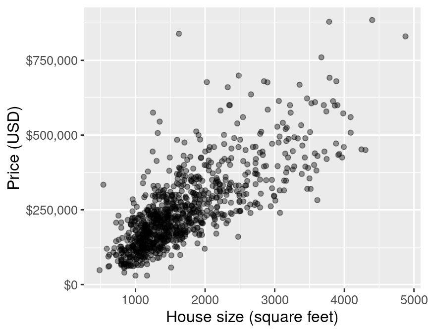
Figure 7.1: Scatter plot of price (USD) versus house size (square feet).
The plot is shown in Figure 7.1. We can see that in Sacramento, CA, as the size of a house increases, so does its sale price. Thus, we can reason that we may be able to use the size of a not-yet-sold house (for which we don’t know the sale price) to predict its final sale price. Note that we do not suggest here that a larger house size causes a higher sale price; just that house price tends to increase with house size, and that we may be able to use the latter to predict the former.
7.5 K-nearest neighbors regression
Much like in the case of classification, we can use a K-nearest neighbors-based approach in regression to make predictions. Let’s take a small sample of the data in Figure 7.1 and walk through how K-nearest neighbors (K-NN) works in a regression context before we dive in to creating our model and assessing how well it predicts house sale price. This subsample is taken to allow us to illustrate the mechanics of K-NN regression with a few data points; later in this chapter we will use all the data.
To take a small random sample of size 30, we’ll use the function
slice_sample, and input the data frame to sample from and the number of rows
to randomly select.
Next let’s say we come across a 2,000 square-foot house in Sacramento we are interested in purchasing, with an advertised list price of $350,000. Should we offer to pay the asking price for this house, or is it overpriced and we should offer less? Absent any other information, we can get a sense for a good answer to this question by using the data we have to predict the sale price given the sale prices we have already observed. But in Figure 7.2, you can see that we have no observations of a house of size exactly 2,000 square feet. How can we predict the sale price?
small_plot <- ggplot(small_sacramento, aes(x = sqft, y = price)) +
  geom_point() +
  xlab("House size (square feet)") +
  ylab("Price (USD)") +
  scale_y_continuous(labels = dollar_format()) +
  geom_vline(xintercept = 2000, linetype = "dashed") +
  theme(text = element_text(size = 12))

small_plot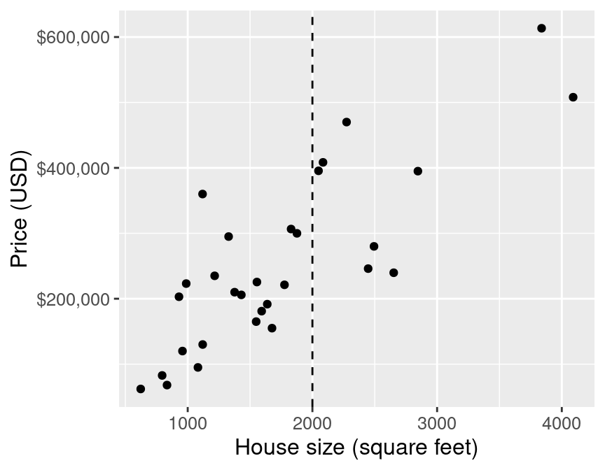
Figure 7.2: Scatter plot of price (USD) versus house size (square feet) with vertical line indicating 2,000 square feet on x-axis.
We will employ the same intuition from the classification chapter, and use the neighboring points to the new point of interest to suggest/predict what its sale price might be. For the example shown in Figure 7.2, we find and label the 5 nearest neighbors to our observation of a house that is 2,000 square feet.
nearest_neighbors <- small_sacramento |>
  mutate(diff = abs(2000 - sqft)) |>
  slice_min(diff, n = 5)

nearest_neighbors
## # A tibble: 5 × 10
## city zip beds baths sqft type price latitude longitude diff
## <chr> <chr> <dbl> <dbl> <dbl> <chr> <dbl> <dbl> <dbl> <dbl>
## 1 ROSEVILLE z95661 3 2 2049 Residenti… 395500 38.7 -121. 49
## 2 ANTELOPE z95843 4 3 2085 Residenti… 408431 38.7 -121. 85
## 3 SACRAMENTO z95823 4 2 1876 Residenti… 299940 38.5 -121. 124
## 4 ROSEVILLE z95747 3 2.5 1829 Residenti… 306500 38.8 -121. 171
## 5 SACRAMENTO z95825 4 2 1776 Multi_Fam… 221250 38.6 -121. 224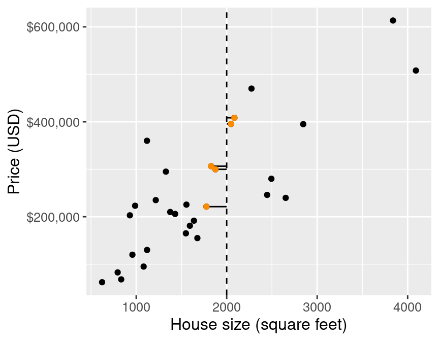
Figure 7.3: Scatter plot of price (USD) versus house size (square feet) with lines to 5 nearest neighbors (highlighted in orange).
Figure 7.3 illustrates the difference between the house sizes of the 5 nearest neighbors (in terms of house size) to our new 2,000 square-foot house of interest. Now that we have obtained these nearest neighbors, we can use their values to predict the sale price for the new home. Specifically, we can take the mean (or average) of these 5 values as our predicted value, as illustrated by the red point in Figure 7.4.
## # A tibble: 1 × 1
##   predicted
##       <dbl>
## 1   326324.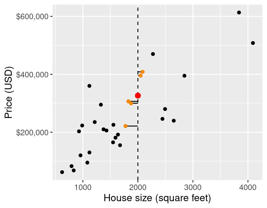
Figure 7.4: Scatter plot of price (USD) versus house size (square feet) with predicted price for a 2,000 square-foot house based on 5 nearest neighbors represented as a red dot.
Our predicted price is $326,324 (shown as a red point in Figure 7.4), which is much less than $350,000; perhaps we might want to offer less than the list price at which the house is advertised. But this is only the very beginning of the story. We still have all the same unanswered questions here with K-NN regression that we had with K-NN classification: which \(K\) do we choose, and is our model any good at making predictions? In the next few sections, we will address these questions in the context of K-NN regression.
One strength of the K-NN regression algorithm that we would like to draw attention to at this point is its ability to work well with non-linear relationships (i.e., if the relationship is not a straight line). This stems from the use of nearest neighbors to predict values. The algorithm really has very few assumptions about what the data must look like for it to work.
7.6 Training, evaluating, and tuning the model
As usual, we must start by putting some test data away in a lock box that we will come back to only after we choose our final model. Let’s take care of that now. Note that for the remainder of the chapter we’ll be working with the entire Sacramento data set, as opposed to the smaller sample of 30 points that we used earlier in the chapter (Figure 7.2).
sacramento_split <- initial_split(sacramento, prop = 0.75, strata = price)
sacramento_train <- training(sacramento_split)
sacramento_test <- testing(sacramento_split)
Next, we’ll use cross-validation to choose \(K\). In K-NN classification, we used accuracy to see how well our predictions matched the true labels. We cannot use the same metric in the regression setting, since our predictions will almost never exactly match the true response variable values. Therefore in the context of K-NN regression we will use root mean square prediction error (RMSPE) instead. The mathematical formula for calculating RMSPE is:
\[\text{RMSPE} = \sqrt{\frac{1}{n}\sum\limits_{i=1}^{n}(y_i - \hat{y}_i)^2}\]
where:
- \(n\) is the number of observations,
- \(y_i\) is the observed value for the \(i^\text{th}\) observation, and
- \(\hat{y}_i\) is the forecasted/predicted value for the \(i^\text{th}\) observation.
In other words, we compute the squared difference between the predicted and true response value for each observation in our test (or validation) set, compute the average, and then finally take the square root. The reason we use the squared difference (and not just the difference) is that the differences can be positive or negative, i.e., we can overshoot or undershoot the true response value. Figure 7.5 illustrates both positive and negative differences between predicted and true response values. So if we want to measure error—a notion of distance between our predicted and true response values—we want to make sure that we are only adding up positive values, with larger positive values representing larger mistakes. If the predictions are very close to the true values, then RMSPE will be small. If, on the other-hand, the predictions are very different from the true values, then RMSPE will be quite large. When we use cross-validation, we will choose the \(K\) that gives us the smallest RMSPE.
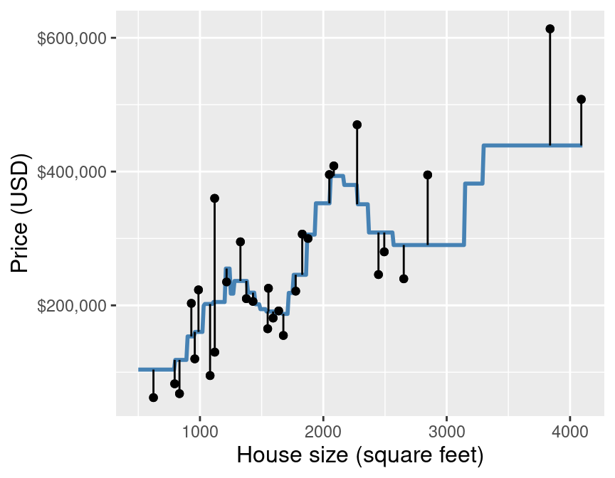
Figure 7.5: Scatter plot of price (USD) versus house size (square feet) with example predictions (blue line) and the error in those predictions compared with true response values (vertical lines).
Note: When using many code packages (
tidymodelsincluded), the evaluation output we will get to assess the prediction quality of our K-NN regression models is labeled “RMSE”, or “root mean squared error”. Why is this so, and why not RMSPE? In statistics, we try to be very precise with our language to indicate whether we are calculating the prediction error on the training data (in-sample prediction) versus on the testing data (out-of-sample prediction). When predicting and evaluating prediction quality on the training data, we say RMSE. By contrast, when predicting and evaluating prediction quality on the testing or validation data, we say RMSPE. The equation for calculating RMSE and RMSPE is exactly the same; all that changes is whether the \(y\)s are training or testing data. But many people just use RMSE for both, and rely on context to denote which data the root mean squared error is being calculated on.
Now that we know how we can assess how well our model predicts a numerical
value, let’s use R to perform cross-validation and to choose the optimal \(K\).
First, we will create a recipe for preprocessing our data.
Note that we include standardization
in our preprocessing to build good habits, but since we only have one
predictor, it is technically not necessary; there is no risk of comparing two predictors
of different scales.
Next we create a model specification for K-nearest neighbors regression. Note
that we use set_mode("regression")
now in the model specification to denote a regression problem, as opposed to the classification
problems from the previous chapters.
The use of set_mode("regression") essentially
tells tidymodels that we need to use different metrics (RMSPE, not accuracy)
for tuning and evaluation.
Then we create a 5-fold cross-validation object, and put the recipe and model specification together
in a workflow.
sacr_recipe <- recipe(price ~ sqft, data = sacramento_train) |>
  step_scale(all_predictors()) |>
  step_center(all_predictors())

sacr_spec <- nearest_neighbor(weight_func = "rectangular",
                              neighbors = tune()) |>
  set_engine("kknn") |>
  set_mode("regression")

sacr_vfold <- vfold_cv(sacramento_train, v = 5, strata = price)

sacr_wkflw <- workflow() |>
  add_recipe(sacr_recipe) |>
  add_model(sacr_spec)

sacr_wkflw
## ══ Workflow ══════════
## Preprocessor: Recipe
## Model: nearest_neighbor()
##
## ── Preprocessor ──────────
## 2 Recipe Steps
##
## • step_scale()
## • step_center()
##
## ── Model ──────────
## K-Nearest Neighbor Model Specification (regression)
##
## Main Arguments:
## neighbors = tune()
## weight_func = rectangular
##
## Computational engine: kknnNext we run cross-validation for a grid of numbers of neighbors ranging from 1 to 200.
The following code tunes
the model and returns the RMSPE for each number of neighbors. In the output of the sacr_results
results data frame, we see that the neighbors variable contains the value of \(K\),
the mean (mean) contains the value of the RMSPE estimated via cross-validation,
and the standard error (std_err) contains a value corresponding to a measure of how uncertain we are in the mean value. A detailed treatment of this
is beyond the scope of this chapter; but roughly, if your estimated mean RMSPE is $100,000 and standard
error is $1,000, you can expect the true RMSPE to be somewhere roughly between $99,000 and $101,000 (although it may
fall outside this range). You may ignore the other columns in the metrics data frame,
as they do not provide any additional insight.
gridvals <- tibble(neighbors = seq(from = 1, to = 200, by = 3))

sacr_results <- sacr_wkflw |>
  tune_grid(resamples = sacr_vfold, grid = gridvals) |>
  collect_metrics() |>
  filter(.metric == "rmse")

# show the results
sacr_results
## # A tibble: 67 × 7
## neighbors .metric .estimator mean n std_err .config
## <dbl> <chr> <chr> <dbl> <int> <dbl> <chr>
## 1 1 rmse standard 107206. 5 4102. Preprocessor1_Model01
## 2 4 rmse standard 90469. 5 3312. Preprocessor1_Model02
## 3 7 rmse standard 86580. 5 3062. Preprocessor1_Model03
## 4 10 rmse standard 85321. 5 3395. Preprocessor1_Model04
## 5 13 rmse standard 85045. 5 3641. Preprocessor1_Model05
## 6 16 rmse standard 84675. 5 3679. Preprocessor1_Model06
## 7 19 rmse standard 84776. 5 3984. Preprocessor1_Model07
## 8 22 rmse standard 84617. 5 3952. Preprocessor1_Model08
## 9 25 rmse standard 84953. 5 3929. Preprocessor1_Model09
## 10 28 rmse standard 84612. 5 3917. Preprocessor1_Model10
## # ℹ 57 more rows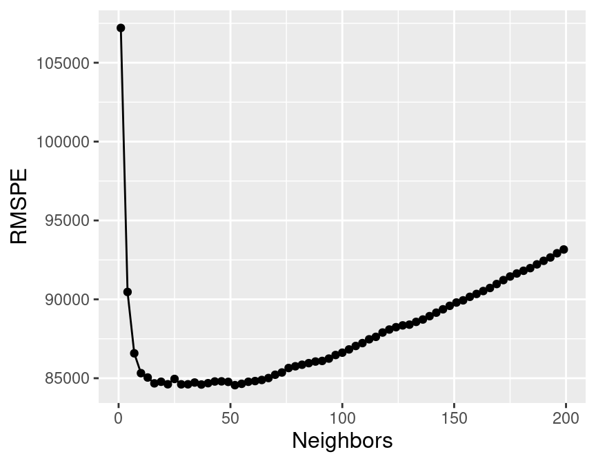
Figure 7.6: Effect of the number of neighbors on the RMSPE.
Figure 7.6 visualizes how the RMSPE varies with the number of neighbors \(K\). We take the minimum RMSPE to find the best setting for the number of neighbors:
## # A tibble: 1 × 7
##   neighbors .metric .estimator   mean     n std_err .config
##       <dbl> <chr>   <chr>       <dbl> <int>   <dbl> <chr>
## 1        52 rmse    standard   84561.     5   4470. Preprocessor1_Model18
The smallest RMSPE occurs when \(K =\) 52.
7.7 Underfitting and overfitting
Similar to the setting of classification, by setting the number of neighbors to be too small or too large, we cause the RMSPE to increase, as shown in Figure 7.6. What is happening here?
Figure 7.7 visualizes the effect of different settings of \(K\) on the regression model. Each plot shows the predicted values for house sale price from our K-NN regression model on the training data for 6 different values for \(K\): 1, 3, 25, 52, 250, and 680 (almost the entire training set). For each model, we predict prices for the range of possible home sizes we observed in the data set (here 500 to 5,000 square feet) and we plot the predicted prices as a blue line.
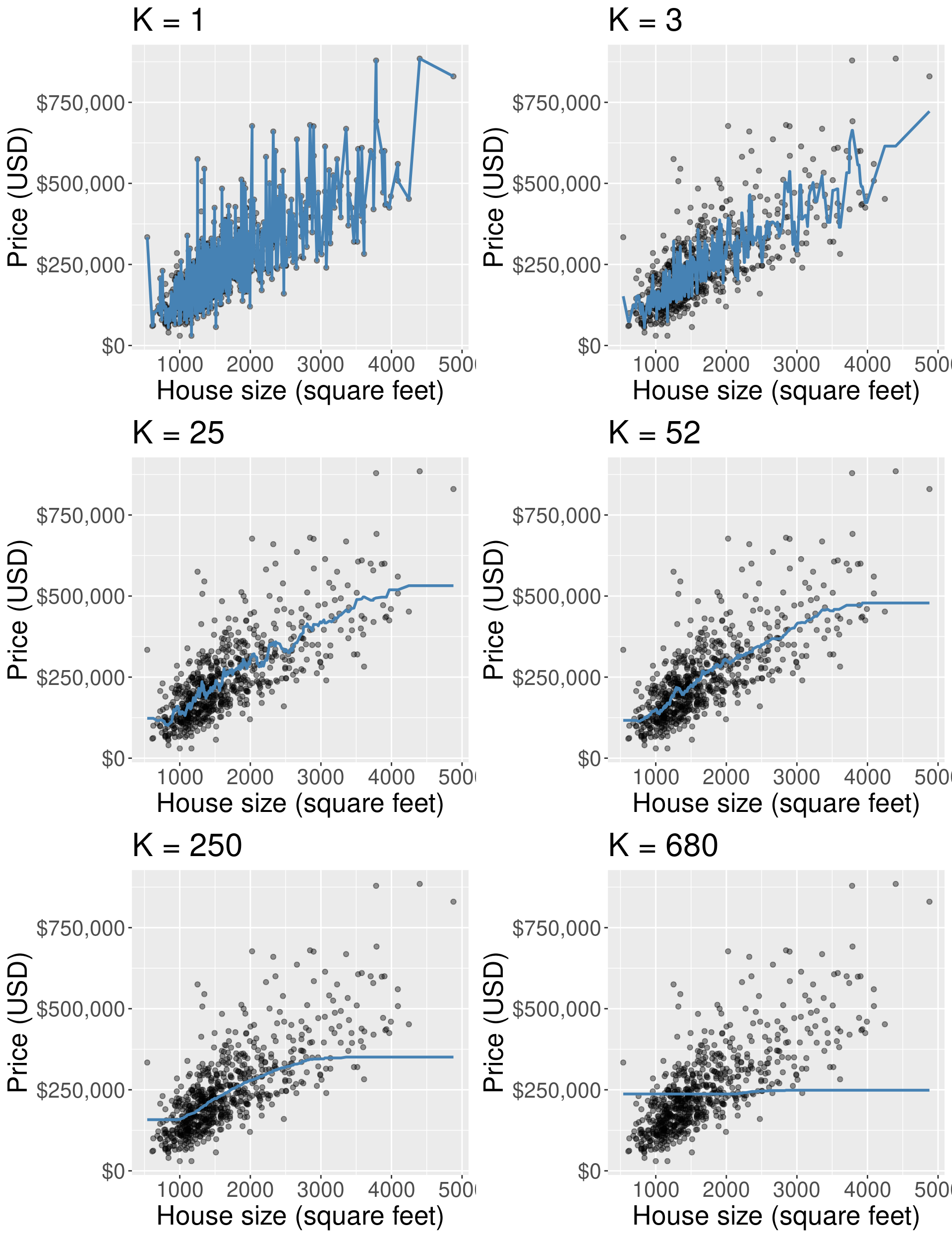
Figure 7.7: Predicted values for house price (represented as a blue line) from K-NN regression models for six different values for \(K\).
Figure 7.7 shows that when \(K\) = 1, the blue line runs perfectly through (almost) all of our training observations. This happens because our predicted values for a given region (typically) depend on just a single observation. In general, when \(K\) is too small, the line follows the training data quite closely, even if it does not match it perfectly. If we used a different training data set of house prices and sizes from the Sacramento real estate market, we would end up with completely different predictions. In other words, the model is influenced too much by the data. Because the model follows the training data so closely, it will not make accurate predictions on new observations which, generally, will not have the same fluctuations as the original training data. Recall from the classification chapters that this behavior—where the model is influenced too much by the noisy data—is called overfitting; we use this same term in the context of regression.
What about the plots in Figure 7.7 where \(K\) is quite large, say, \(K\) = 250 or 680? In this case the blue line becomes extremely smooth, and actually becomes flat once \(K\) is equal to the number of datapoints in the training set. This happens because our predicted values for a given x value (here, home size), depend on many neighboring observations; in the case where \(K\) is equal to the size of the training set, the prediction is just the mean of the house prices (completely ignoring the house size). In contrast to the \(K=1\) example, the smooth, inflexible blue line does not follow the training observations very closely. In other words, the model is not influenced enough by the training data. Recall from the classification chapters that this behavior is called underfitting; we again use this same term in the context of regression.
Ideally, what we want is neither of the two situations discussed above. Instead, we would like a model that (1) follows the overall “trend” in the training data, so the model actually uses the training data to learn something useful, and (2) does not follow the noisy fluctuations, so that we can be confident that our model will transfer/generalize well to other new data. If we explore the other values for \(K\), in particular \(K\) = 52 (as suggested by cross-validation), we can see it achieves this goal: it follows the increasing trend of house price versus house size, but is not influenced too much by the idiosyncratic variations in price. All of this is similar to how the choice of \(K\) affects K-nearest neighbors classification, as discussed in the previous chapter.
7.8 Evaluating on the test set
To assess how well our model might do at predicting on unseen data, we will
assess its RMSPE on the test data. To do this, we will first
re-train our K-NN regression model on the entire training data set,
using \(K =\) 52 neighbors. Then we will
use predict to make predictions on the test data, and use the metrics
function again to compute the summary of regression quality. Because
we specify that we are performing regression in set_mode, the metrics
function knows to output a quality summary related to regression, and not, say, classification.
kmin <- sacr_min |> pull(neighbors)

sacr_spec <- nearest_neighbor(weight_func = "rectangular", neighbors = kmin) |>
  set_engine("kknn") |>
  set_mode("regression")

sacr_fit <- workflow() |>
  add_recipe(sacr_recipe) |>
  add_model(sacr_spec) |>
  fit(data = sacramento_train)

sacr_summary <- sacr_fit |>
  predict(sacramento_test) |>
  bind_cols(sacramento_test) |>
  metrics(truth = price, estimate = .pred) |>
  filter(.metric == 'rmse')

sacr_summary
## # A tibble: 1 × 3
## .metric .estimator .estimate
## <chr> <chr> <dbl>
## 1 rmse standard 90529.Our final model’s test error as assessed by RMSPE is $90,529. Note that RMSPE is measured in the same units as the response variable. In other words, on new observations, we expect the error in our prediction to be roughly $90,529. From one perspective, this is good news: this is about the same as the cross-validation RMSPE estimate of our tuned model (which was $84,561), so we can say that the model appears to generalize well to new data that it has never seen before. However, much like in the case of K-NN classification, whether this value for RMSPE is good—i.e., whether an error of around $90,529 is acceptable—depends entirely on the application. In this application, this error is not prohibitively large, but it is not negligible either; $90,529 might represent a substantial fraction of a home buyer’s budget, and could make or break whether or not they could afford put an offer on a house.
Finally, Figure 7.8 shows the predictions that our final model makes across the range of house sizes we might encounter in the Sacramento area. Note that instead of predicting the house price only for those house sizes that happen to appear in our data, we predict it for evenly spaced values between the minimum and maximum in the data set (roughly 500 to 5000 square feet). We superimpose this prediction line on a scatter plot of the original housing price data, so that we can qualitatively assess if the model seems to fit the data well. You have already seen a few plots like this in this chapter, but here we also provide the code that generated it as a learning opportunity.
sqft_prediction_grid <- tibble(
    sqft = seq(
        from = sacramento |> select(sqft) |> min(),
        to = sacramento |> select(sqft) |> max(),
        by = 10
    )
)

sacr_preds <- sacr_fit |>
  predict(sqft_prediction_grid) |>
  bind_cols(sqft_prediction_grid)

plot_final <- ggplot(sacramento, aes(x = sqft, y = price)) +
  geom_point(alpha = 0.4) +
  geom_line(data = sacr_preds,
            mapping = aes(x = sqft, y = .pred),
            color = "steelblue",
            linewidth = 1) +
  xlab("House size (square feet)") +
  ylab("Price (USD)") +
  scale_y_continuous(labels = dollar_format()) +
  ggtitle(paste0("K = ", kmin)) +
  theme(text = element_text(size = 12))

plot_final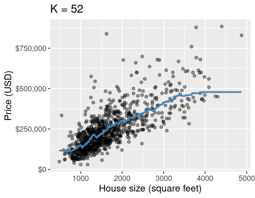
Figure 7.8: Predicted values of house price (blue line) for the final K-NN regression model.
7.9 Multivariable K-NN regression
As in K-NN classification, we can use multiple predictors in K-NN regression.
In this setting, we have the same concerns regarding the scale of the predictors. Once again,
predictions are made by identifying the \(K\)
observations that are nearest to the new point we want to predict; any
variables that are on a large scale will have a much larger effect than
variables on a small scale. But since the recipe we built above scales and centers
all predictor variables, this is handled for us.
Note that we also have the same concern regarding the selection of predictors in K-NN regression as in K-NN classification: having more predictors is not always better, and the choice of which predictors to use has a potentially large influence on the quality of predictions. Fortunately, we can use the predictor selection algorithm from the classification chapter in K-NN regression as well. As the algorithm is the same, we will not cover it again in this chapter.
We will now demonstrate a multivariable K-NN regression analysis of the
Sacramento real estate data using tidymodels. This time we will use
house size (measured in square feet) as well as number of bedrooms as our
predictors, and continue to use house sale price as our response variable
that we are trying to predict.
It is always a good practice to do exploratory data analysis, such as
visualizing the data, before we start modeling the data. Figure 7.9
shows that the number of bedrooms might provide useful information
to help predict the sale price of a house.
plot_beds <- sacramento |>
  ggplot(aes(x = beds, y = price)) +
  geom_point(alpha = 0.4) +
  labs(x = 'Number of Bedrooms', y = 'Price (USD)') +
  theme(text = element_text(size = 12))
plot_beds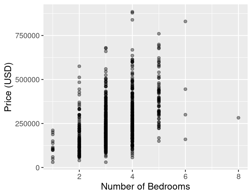
Figure 7.9: Scatter plot of the sale price of houses versus the number of bedrooms.
Figure 7.9 shows that as the number of bedrooms increases, the house sale price tends to increase as well, but that the relationship is quite weak. Does adding the number of bedrooms to our model improve our ability to predict price? To answer that question, we will have to create a new K-NN regression model using house size and number of bedrooms, and then we can compare it to the model we previously came up with that only used house size. Let’s do that now!
First we’ll build a new model specification and recipe for the analysis. Note that
we use the formula price ~ sqft + beds to denote that we have two predictors,
and set neighbors = tune() to tell tidymodels to tune the number of neighbors for us.
sacr_recipe <- recipe(price ~ sqft + beds, data = sacramento_train) |>
  step_scale(all_predictors()) |>
  step_center(all_predictors())
sacr_spec <- nearest_neighbor(weight_func = "rectangular",
                              neighbors = tune()) |>
  set_engine("kknn") |>
  set_mode("regression")
Next, we’ll use 5-fold cross-validation to choose the number of neighbors via the minimum RMSPE:
gridvals <- tibble(neighbors = seq(1, 200))

sacr_multi <- workflow() |>
  add_recipe(sacr_recipe) |>
  add_model(sacr_spec) |>
  tune_grid(sacr_vfold, grid = gridvals) |>
  collect_metrics() |>
  filter(.metric == "rmse") |>
  filter(mean == min(mean))

sacr_k <- sacr_multi |>
              pull(neighbors)
sacr_multi
## # A tibble: 1 × 7
## neighbors .metric .estimator mean n std_err .config
## <int> <chr> <chr> <dbl> <int> <dbl> <chr>
## 1 11 rmse standard 81839. 5 3108. Preprocessor1_Model011Here we see that the smallest estimated RMSPE from cross-validation occurs when \(K =\) 11. If we want to compare this multivariable K-NN regression model to the model with only a single predictor as part of the model tuning process (e.g., if we are running forward selection as described in the chapter on evaluating and tuning classification models), then we must compare the RMSPE estimated using only the training data via cross-validation. Looking back, the estimated cross-validation RMSPE for the single-predictor model was $84,561. The estimated cross-validation RMSPE for the multivariable model is $81,839. Thus in this case, we did not improve the model by a large amount by adding this additional predictor.
Regardless, let’s continue the analysis to see how we can make predictions with a multivariable K-NN regression model and evaluate its performance on test data. We first need to re-train the model on the entire training data set with \(K =\) 11, and then use that model to make predictions on the test data.
sacr_spec <- nearest_neighbor(weight_func = "rectangular",
                              neighbors = sacr_k) |>
  set_engine("kknn") |>
  set_mode("regression")

knn_mult_fit <- workflow() |>
  add_recipe(sacr_recipe) |>
  add_model(sacr_spec) |>
  fit(data = sacramento_train)

knn_mult_preds <- knn_mult_fit |>
  predict(sacramento_test) |>
  bind_cols(sacramento_test)

knn_mult_mets <- metrics(knn_mult_preds, truth = price, estimate = .pred) |>
                     filter(.metric == 'rmse')

knn_mult_mets
## # A tibble: 1 × 3
## .metric .estimator .estimate
## <chr> <chr> <dbl>
## 1 rmse standard 90862.This time, when we performed K-NN regression on the same data set, but also included number of bedrooms as a predictor, we obtained a RMSPE test error of $90,862. Figure 7.10 visualizes the model’s predictions overlaid on top of the data. This time the predictions are a surface in 3D space, instead of a line in 2D space, as we have 2 predictors instead of 1.
Figure 7.10: K-NN regression model’s predictions represented as a surface in 3D space overlaid on top of the data using three predictors (price, house size, and the number of bedrooms). Note that in general we recommend against using 3D visualizations; here we use a 3D visualization only to illustrate what the surface of predictions looks like for learning purposes.
We can see that the predictions in this case, where we have 2 predictors, form a surface instead of a line. Because the newly added predictor (number of bedrooms) is related to price (as price changes, so does number of bedrooms) and is not totally determined by house size (our other predictor), we get additional and useful information for making our predictions. For example, in this model we would predict that the cost of a house with a size of 2,500 square feet generally increases slightly as the number of bedrooms increases. Without having the additional predictor of number of bedrooms, we would predict the same price for these two houses.
7.10 Strengths and limitations of K-NN regression
As with K-NN classification (or any prediction algorithm for that matter), K-NN regression has both strengths and weaknesses. Some are listed here:
Strengths: K-nearest neighbors regression
- is a simple, intuitive algorithm,
- requires few assumptions about what the data must look like, and
- works well with non-linear relationships (i.e., if the relationship is not a straight line).
Weaknesses: K-nearest neighbors regression
- becomes very slow as the training data gets larger,
- may not perform well with a large number of predictors, and
- may not predict well beyond the range of values input in your training data.
7.11 Exercises
Practice exercises for the material covered in this chapter can be found in the accompanying worksheets repository in the “Regression I: K-nearest neighbors” row. You can launch an interactive version of the worksheet in your browser by clicking the “launch binder” button. You can also preview a non-interactive version of the worksheet by clicking “view worksheet.” If you instead decide to download the worksheet and run it on your own machine, make sure to follow the instructions for computer setup found in Chapter 13. This will ensure that the automated feedback and guidance that the worksheets provide will function as intended.
 Data Science